


![]() n two-dimensional MR imaging, a slice is excited, for example, by applying a selective RF-pulse in the presence of the z-gradient. Two different methods can be applied.
n two-dimensional MR imaging, a slice is excited, for example, by applying a selective RF-pulse in the presence of the z-gradient. Two different methods can be applied.
The remaining two gradients (x and y) are now combined with a resulting gradient of a certain strength and spatial direction. The FID is recorded in the presence of this gradient. Then the combined gradient is rotated a certain angle. Once again the FID is recorded, and this process continues until enough information is collected.
Based on the frequency spectra, an image can be reconstructed using the backprojection method, as depicted in Figure 06-13.
This method is a combination of phase- and frequency-encoding. It is the standard image formation method today.
One gradient, for example the y-gradient, is switched on and the spins are allowed to dephase in the presence of this gradient. After a certain time, the y-gradient is switched off and the FID, or alternatively the spin echo, is recorded in the presence of the x-gradient.
Thus, the y-gradient serves as the phase-encoding gradient (often called preparation gradient) and the x-gradient is encoding the frequency information (readout gradient). The system is re-excited, but with either the duration or, more commonly, the strength of the y-gradient changed.
The whole process is repeated n times for a resolution of n pixels in the y-direction, with a different phase-encoding gradient applied for each excitation.
Since the field inhomogeneity effects will be the same for each repetition, they have no effect upon the final image; rather, they constitute a baseline. This is one of the main advantages of the 2DFT technique.
The resulting 2D raw data matrix is processed using a 2D Fourier-transform to produce a 2D image (Figure 06-20) [⇒ Pykett 1982]. The combination of frequency- and amplitude-stepped phase-encoding techniques is called 2D spin warp imaging [⇒ Edelstein 1980].
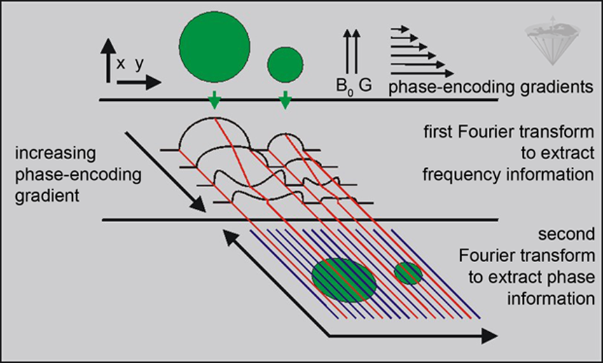
Figure 06-20:
2DFT owes more to MR spectroscopy than to CT reconstruction algorithms because both amplitude and phase information are acquired to spatially encode the signal.
The first step generates a one-dimensional projection, but here a phase-encoding gradient is applied just before the original gradient is turned on. The phase-encoding gradient is applied in right angles to the original gradient and its duration or amplitude is successively increased. The corresponding points from each projection are Fourier-transformed a second time to generate the final image.
Figure 06-21 summarizes an entire 2DFT imaging experiment, in this case using a spin-echo sequence, although one can use nearly any other pulse sequence applied in clinical MR imaging.
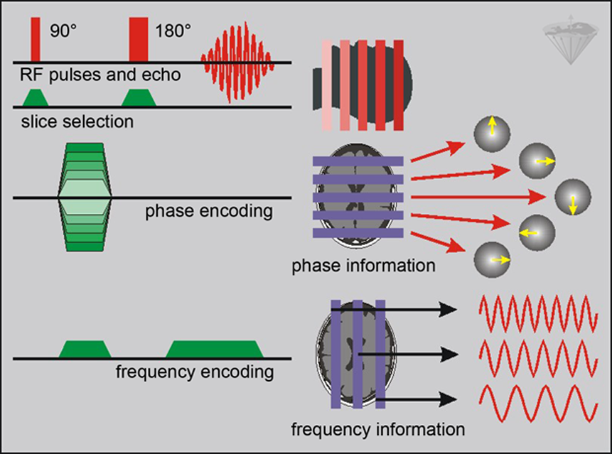
Figure 06-21:
Complete 2DFT SE imaging experiment. The procedure consists of the selection of the 90° and 180° RF pulses, a transverse slice through a brain (z-direction), phase-encoding (y-direction), and frequency-encoding (x-direction).
The phase-encoding gradients change the phase in the respective row of the transverse slice; the frequency-encoding gradients allocate a specific frequency to each column. Combining both phase and frequency information allows the creation of a grid in which each pixel possesses a distinct combination of phase and frequency codes. The entire procedure is usually repeated 256 times, with changing phase-encoding gradients to produce a 256×256 image.


|

|
|---|