


![]() n radiology, the times of conventional imaging ended in September 1971 when the world's first axial x-ray computer assisted tomograph (CT or CAT) was installed in England.
n radiology, the times of conventional imaging ended in September 1971 when the world's first axial x-ray computer assisted tomograph (CT or CAT) was installed in England.
In the same month, on 2 September 1971, Paul C. Lauterbur, a professor of chemistry at the State University of New York at Stony Brook (Figure 20-24), recorded in his laboratory notebook the idea of applying magnetic field gradients in all three dimensions to create NMR images — and had his invention certified (Figure 20-25); yet, he was never able to patent it — the president, administrators and lawyers of the university did not believe that the technique would have any future.
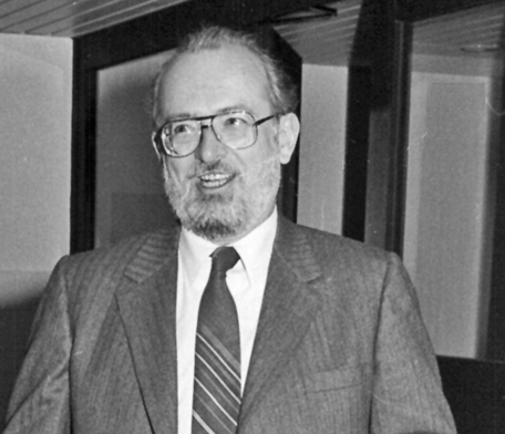
Figure 20-24:
Paul C. Lauterbur (1929-2007).
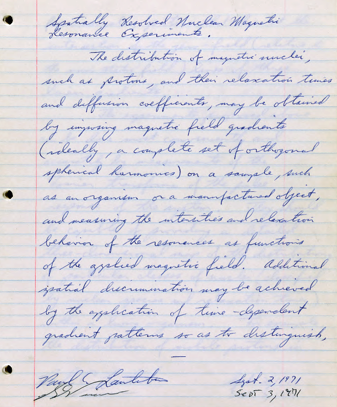
Figure 20-25:
First page of Lauterbur's laboratory notebook describing his idea of "Spatially resolved nuclear magnetic resonance experiments," signed and witnessed on 3 September 1971.
Already in the 1950s and 1960s Lauterbur had established his fame in the community of nuclear magnetic resonance scientists by showing carbon and silicon spectra which led to many publications on various classes of organic chemicals [⇒ Lauterbur 1957].
However, all experiments before Lauterbur's invention of 1971 had been one-dimensional and lacked spatial information. Nobody could determine exactly where the NMR signal originated within the sample. Lauterbur's idea changed this.
Lauterbur called his imaging method zeugmatography, combining the Greek words "zeugma" (ζεῦγμα = the bridge or the yoke that holds two animals together in front of a carriage) and "graphein" (γράφειν = to write, to depict) to describe the joining of chemical and spatial information. This term was later replaced by (N)MR imaging or MRI. A graphic depiction from 1978 of what would become the first whole-body MR apparatus at his laboratory is shown on Figure 03-01.
He published the first images of two tubes of water in March 1973 in Nature (Figure 20-26) [⇒ Lauterbur 1973]. Later in the year the picture of a living animal, a clam, followed and in 1974 the image of the thoracic cavity of a mouse [⇒ Lauterbur 1974].
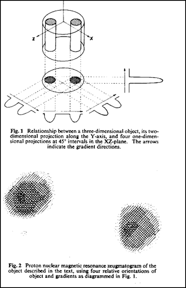
Figure 20-26:
Lauterbur’s first published MR images acquired at the State University of New York at Stony Brook (from Nature 1973; 242: 190-191; reprinted with permission).
Many of today's innovations were thought of and developed in Lauterbur's laboratory in the late 1970s and 1980s, from radio-frequency coil design, magnetization transfer, 3D- as well as chemical shift imaging, heart and lung imaging, using elements different from hydrogen, to NMR microscopy and contrast agents, oblique and curved slice reconstructions, and flow imaging [⇒ Bernardo 1982; ⇒ Frank 1976; ⇒ Lai 1980; ⇒ Lauterbur 1974; 1975; 1976; 1977; 1978; ⇒ Muller 1983; ⇒ Rinck 1984; ⇒ Simon 1981].
Some early examples are shown in Figure 20-27.
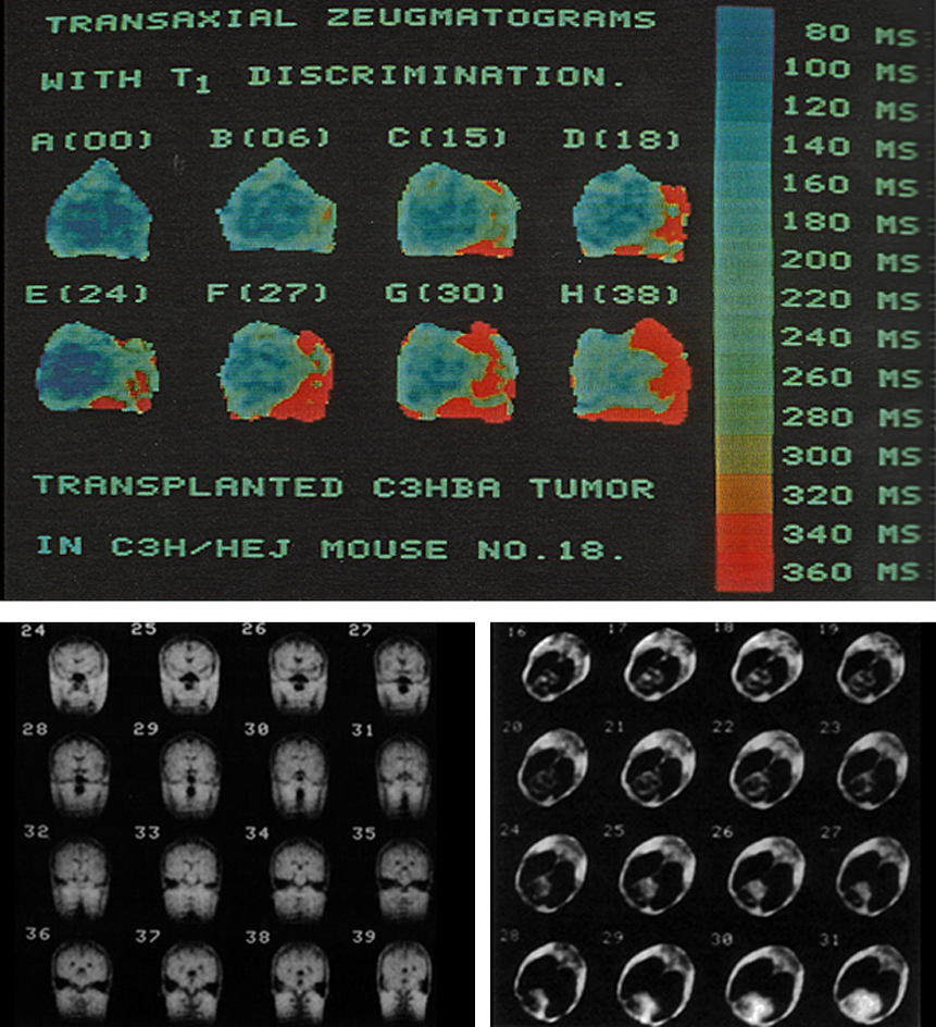
Figure 20-27:
Early examples of “zeugmatography”. These images were made in 1982.
Top: Follow-up of the growth of an implanted tumor in a mouse for a period of 38 days. Each image was resonstructed from 12 projection, the slice thickness was about 3 cm.
Later, most images in Lauterbur's laboratory were acquired in three dimensions. 3D-imaging with commercial systems became only possible some 10 years later.
Bottom left: Coronal images from a 3D human brain study.
Bottom right: Transverse images from a 3D study of a dog's heart, synchronized with the ECG, 400 ms after the R-wave.
Field gradients had been used before, though only in one dimension and without imaging in the mind of the researchers.
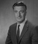 Figure 20-28: Erwin Louis Hahn (1921-2016).
They are an essential feature of the study of molecular diffusion in liquids by the spin-echo method developed by Erwin L. Hahn in 1950 (Figure 20-28) [⇒ Hahn 1950]; his group also used a gradient approach to create a storage memory [⇒ Anderson 1955].
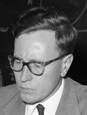 Figure 20-29: Robert Gabillard (1926-2012).
In 1951, Robert Gabillard (Figure 20-29) from Lille in France had imposed one-dimensional gradients on samples [⇒ Gabillard 1951; 1952].
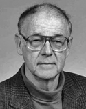 Figure 20-30: Herman Y. Carr (1924-2008).
Herman Y. Carr (Figure 20-30) and Edward M. Purcell described the use of gradients in the determination of diffusion in 1954 [⇒ Carr 1954].


|

|
|---|