


![]() n an imaging experiment, definition and selection of a virtual (two-dimensional) slice through the examined object or a patient are of great importance. They are determined by characteristics of the excitation pulse. One distinguishes between shaped and hard pulses (cf. Figure 01-08).
n an imaging experiment, definition and selection of a virtual (two-dimensional) slice through the examined object or a patient are of great importance. They are determined by characteristics of the excitation pulse. One distinguishes between shaped and hard pulses (cf. Figure 01-08).
We can express the gradient strength in either mT/m or in Hz/m. Since the pulse has a fixed bandwidth (provided that the pulse duration is held constant), raising the gradient strength increases the number of Hz/m; this results in a decrease in slice thickness (Figure 06-15).
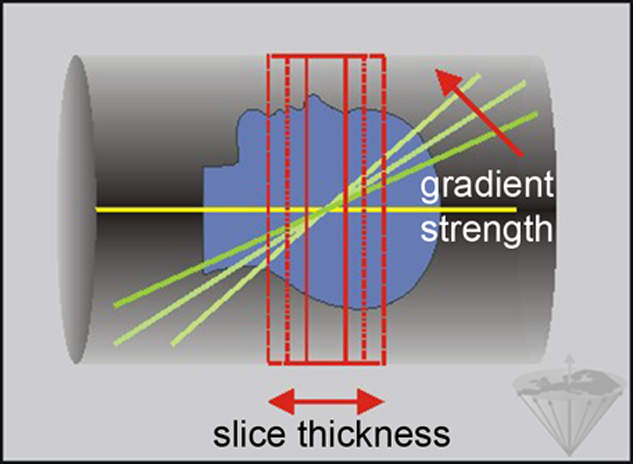
Figure 06-15:
Slice thickness: moving the gradient in the direction of the arrow increases the number of Hz/m, and thus gradient strength. It decreases slice thickness.
For example, for a sinc pulse with a bandwidth of 2 kHz, increasing the slice gradient from 4 mT/m (1.7 kHz/cm) to 8 mT/m (3.4 kHz/cm) reduces the slice thickness from 11.8 mm to 5.9 mm.
Applying an RF pulse in the absence of any field gradients will excite the whole sample. If a field gradient is applied at the same time as the pulse, the magnetic field, and therefore the resonance frequency, will change with position within the sample. For an RF pulse at the resonance frequency excitation will occur at the magnet center where the gradient has no effect (cf. Figure 06-05).
Off-center, the nuclei cannot be excited by RF pulses at the Larmor frequency. The distance (or slice thickness) over which the nuclei in the center resonate is determined by the range of frequencies (bandwidth) contained in the excitation pulse and the strength of the field gradient. If the RF pulse contains only a well defined band of frequencies, then excitation will occur for a well defined range of positions. This excitation corresponds to the selection of a slice in the sample.
 The length of the RF pulse, and thus also its bandwidth, is the second factor influencing the slice thickness. The longer the pulse, the thinner the slice will be (Figure 06-16).
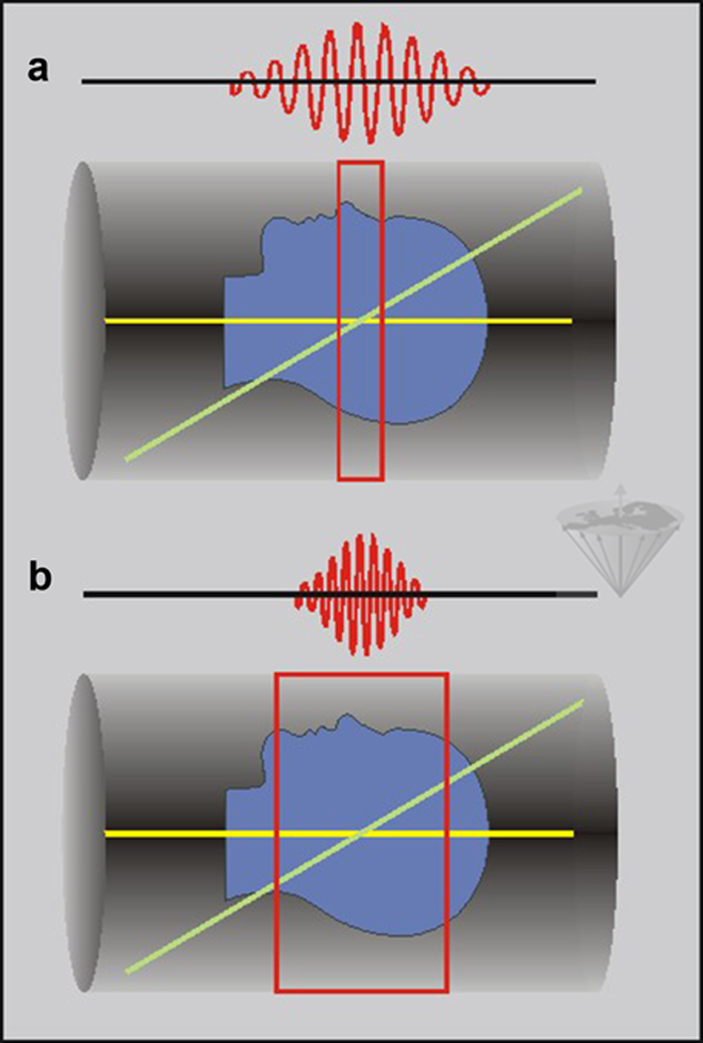
Figure 06-16:
(a) Long sinc pulses lead to thin slices, whereas (b) short sinc pulses increase slice thickness
The trade-off for thinner slices is the prolongation of the echo time (TE). Because TE is measured from the center of the pulse, longer pulses for thinner slices mean a longer initial TE, which, in turn, influences imaging time, image artifacts, and contrast.
Changing the frequency of the RF pulse corresponds to moving the position of the nuclei on resonance from the center of the sample. In this way we can move the slice to any desired location along the axis (Figure 06-17). For a transverse slice, the slice gradient is applied along the z-axis; for a coronal slice, the slice gradient is applied along the y-axis; and for a sagittal slice, it is applied along the x-axis.
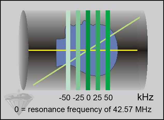
Figure 06-17:
Moving the slice position: at 1.0 T, the resonance frequency in the center of the sample corresponds to 42.57 MHz. Changing the pulse frequency by several kHz moves the slice off-center.
In analytical NMR studies, the maximal RF power is applied for a time sufficiently long to give the desired pulse angle (hard pulse). In more complicated experiments, it is necessary to adjust the pulse amplitude with time so as to give a better defined frequency content (shaped pulse).
The pulse shape is used to give an approximately rectangular slice profile for the slices in the imaging experiments (Gaussian and sinc pulses; see Figure 01-09) and can heavily influence image contrast in magnetic resonance imaging.
The phase of the RF pulse is also determined at this stage, with many MR machines only allowing phases of 0°, 90°, 180° or 270° to be selected. The resulting excitation pulses can be as short as 10 ms for non-selective hard pulses, and typically a few milliseconds for the frequency-selective shaped pulses used in magnetic resonance imaging with peak-to-peak amplitudes of up to several hundred volts.


|

|
|---|