


 ifteen years after the first description of different relaxation behavior in tissues by Erik Odeblad [⇒ Odeblad 1955], other researchers started postulating that relaxation times differentiate tumors from normal tissue since most T1 (and in a similar way T2) values of pathologic tissue can differ markedly from the T1 of the similar normal tissue [⇒ Damadian 1971] (cf. Chapter 20: History of MRI).
However, the ability to discriminate, type, or even grade tumors using relaxation time values has remained a dream, despite the sophisticated multi-point fits introduced over the years. Figure 04-24 shows that there are differences between, in this case, T2 of normal and diseased tissues [⇒ Rinck 1985]. Although values of T2 are more accurate than those of T1 because more points are used for their calculation, these differences are not significant between T2 values of, for instance, tumors and edema or infarction.
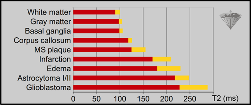
Figure 04-24:
T2 values of normal and pathological human brain tissues measured at 0.15 Tesla, based upon 24 echoes. The standard deviation (SD) is given in yellow. The SD of normal tissues can reach 20%, that of pathological tissues 30%.
Every year, the literature announces new attempts to exploit relaxation-time measurements in vivo. There are some positive reports about its successful use. Many concern follow-up of therapy, with patients being their own reference.
Publications include, for instance, the report that relaxation times from leukemic bone marrow can be used for the differential diagnosis of this disease (Figure 04-25) [⇒ Jensen 1990]. Similar results in high-grade gliomas have been published by another research group [⇒ Boesiger 1990].
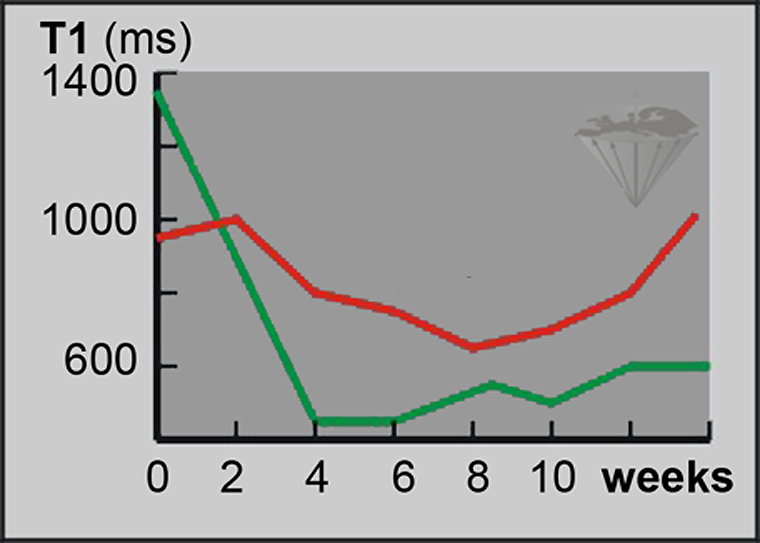
Figure 04-25:
T1 measurements. Follow-up of treatment of acute myeloblastic leukemia.
Green = responder; red = non-responder.
Yet, the follow-up of treatment based upon relaxation-time values is difficult and in most instances dubious (Figure 04-26). A rise and subsequent decline of relaxation time values after a local intervention might rather indicate edema and inflammation than successful treatment [⇒ Zhang 2014].
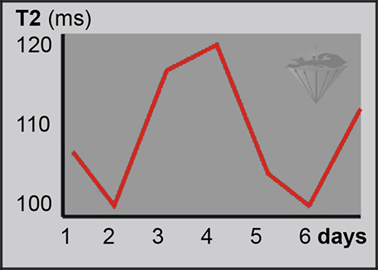
Figure 04-26:
Relaxation-time measurements of identical samples under identical measurement conditions can reveal great standard deviations, as shown in this example.
Relying on in vivo measurements to evaluate the outcome of treatment is dubious. Only in some instances do massive changes allow a positive assessment.
Several other studies dealt with pixel-by-pixel mapping of relaxation times of normal appearing white brain matter in multiple sclerosis (MS) patients. The results suggested minute invisible changes in the white matter which might explain brain function deficits that cannot be explained by the size and location of visible MS plaques [⇒ Barbosa 1994, ⇒ Lacomis 1986, ⇒ Rinck 1987].
However, also these measurements are not clinically applicable.
Availability of databases of in vivo relaxation-time measurements is very limited. A large collection of data was published by Bottomley et al. [⇒ Bottomley 1984, 1987].
A comparison between in vivo and in vitro relaxation measurements is quite difficult because many T1 relaxation time values change rapidly after excision. Only brain tissues reveal a relatively stable relaxation behavior after they have been removed from the body [⇒ Fischer 1989, 1990].
After absolute T1 and T2 values had been used unsuccessfully by researchers, combinations of T1 and T2, histogram techniques, and sophisticated three dimensional display techniques of factor representations were used (‘fingerprinting’, biomarkers) [⇒ Skalej 1985].
Precise measurements require long acquisition times; the repetition time, TR, should be equal to or greater than 5×T1. At 0.15 T, the T1 of myocardium is around 380 ms, at 1.5 T it has climbed to around 1000 ms. Measurements at low fields take approximately 5 minutes, at high or ultrahigh field more than 10, perhaps 15 minutes. Thus, makeshift faster acquisition methods were sought and developed.
Fast acquisition of quantitative T1 maps can, e.g., be based on a series of snapshot fast low-angle shot (FLASH) images after inversion of the magnetization [⇒ Deichmann 1999].
Such techniques were for instance used for estimating the concentration of paramagnetic contrast agents in an organ.
Since the acquisition of quantitative tissue data from a beating heart has to be very fast, lately much research is focused on modifications of a pulsed NMR sequence proposed by David C. Look and Donald R. Locker in 1969. MRI did not exist at that time, and Look and Locker used their time-saving one-shot method for NMR spectroscopy instead of the conventional methods to measure the T1 relaxation time. The spectroscopic “LL” method was within 10% of the conventionally precisely calculated value [⇒ Look 1969].
In the 1980s, the method was further developed for MRI by Graumann and his colleagues [⇒ Graumann 1987].
Others followed and precision was waived for speed. Among the modified sequences for cardiac and, e.g., brain MRI experimentally (and sometimes clinically) used today, one finds PURR [⇒ Lee 2000], MOLLI [⇒ Messroghli 2004], and ShMOLLI [⇒ Piechnik 2010]. They all suffer to varying extent from errors, resulting in an underestimation of the true T1. ‘Apparent’ T1 values of MOLLI and ShMOLLI measurements of, e.g., normal myocardium have an error range of 30% or higher and always are shorter than true T1 values.
A number of different pulse sequences, e.g., SASHA, SAPPHIRE, DESPOT and many others were also introduced and tested. Unfortunately, none of these values are reliable or reproducible (Figure 04-27) [⇒ Bojorquez 2017]. From scientific and medical points of view, these measurements are unsound because the margin of error is huge.
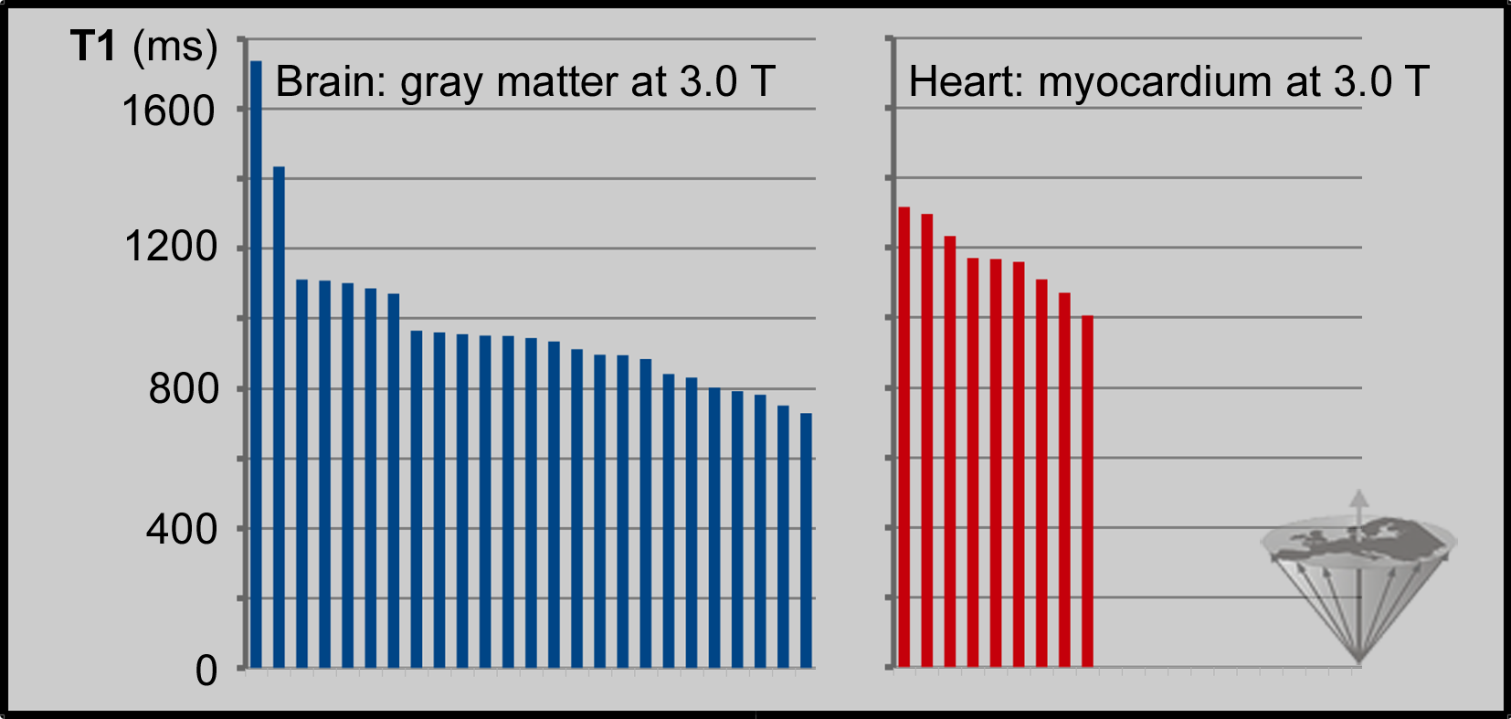
Figure 04-27:
T1 values at 3 Tesla of human gray brain matter (25 different collectives) and myocardium (9 different collectives) measured in vivo on different MR machines with accelerated data acquisition algorithms (compiled from different sources). The estimated values are imprecise and spread across several hundred milliseconds.
The sharp fall of T2* values at high and ultrahigh fields is related to the drastic rise of magnetic susceptibility effects which grow linearly with magnetic field strength; pure T2 is not affected in the same way. Imperfect spoiling of transverse magnetization at higher flip angles in gradient echo sequences has a negative effect on a precise estimation of signal intensity and other parameters, such as relaxation times [⇒ Zur 1991].
 Critical Remarks. Yet, in the end, it is not even the most elaborate data acquisition that makes typing of normal and pathological tissues (‘fingerprinting’) or grading of diseases impossible but rather the complexity of tissue composition and the overlapping of relaxation time values of heterogeneous volume elements examined and processed into a single number or number range.
It is helpful to once look into a microscope and to see how complex and complicate tissue structures are, both in normal and in pathological tissues — and in abnormal, but not (yet) pathological tissues.
Even following a trend of changing T1 and T2 acquired with the same equipment and the same imaging parameters to calculate the relaxation constant values during and after the treatment of a patient can be like 'fishing in troubled waters.'
From a scientific point of view, MR imaging is a crude and not very exact technology. However, to be imprecise in medicine does not preclude specific use.
One example is the measurement of cardiac iron overload, which according to a number of cardiological publications is, so far, one of the most useful diagnostic approaches in patients with thalassemia major; however, many papers about the topic are dubious and the methods used lack scientific background. Myocardial damage in thalassemia is induced by iron deposition: free unbound iron catalyzes the formation of cell-toxic hydroxyl radicals. Thus, monitoring of myocardial iron content would be useful and could be done by estimating T2 or T2*.
To be able to discriminate ‘normal’ myocardium and pathological tissue alteration the approach requires massive tissue changes, and it cannot distinguish between fibrosis, inflammation, and infiltrative cardiomyopathies, myocardial edema and other possible tissue changes. However, the pathological T2* values seem to be highly reproducible on different MR equipment [⇒ Auger 2016].
Another area of application of relaxation times measurements might be the follow-up of massive T1 changes after the injection of a targeted contrast agent, such as Mn-DPDP and the comparison of plain and contrast-enhanced tissue, e.g., in heart diseases (cf. cardiac applications of manganese).
Here, too, imprecise measurements might be of diagnostic value.
To add confusion to complicated science, changes of terms and terminology are common in contemporary bioscience.
Thirty years after the description of relaxation times and relaxation rates as possible or, rather, questionable biological indicators they were re-ranked among biological markers or biomarkers.
In general, biomarkers are biological indicators of any kind; there are thousands of them. They are not specific for MR imaging or MR spectroscopy. Typical biomarkers are measurements or scores such as blood pressure, body temperature, the body mass index, or clinical signs such as external manifestations of disease. Many of them are helpful, others of limited and questionable value — still widely used.
In MR imaging, biomarkers break down into numerous subgroups where they can be applied standing alone or several combined, relaxation times being only one of them.
Aside of T1 and T2, there are other possible indicators for the detection, diagnosis, and monitoring of treatment, i.e., of particular physiological or disease states.
Quantification of MR parameters is also discussed in Chapter 15. Biomarkers extracted through image segmentation and multispectral analysis and the basics of artificial intelligence are also described in Chapter 15, those acquired with the help of contrast agents in Chapter 13, and by dynamic imaging in Chapter 16.


|
Chapter 4 — Page 7 |

|
|---|