


![]() mage contrast is calculable for the conventional pulse sequences, but there are increasingly other ('black box') sequences where contrast is not predictable.
mage contrast is calculable for the conventional pulse sequences, but there are increasingly other ('black box') sequences where contrast is not predictable.
On the following pages, we will first look at the basic pulse sequences and their contrast influencing components TR, TE, TI, FA, and others — step-by-step. Many other pulse sequences can be derived from the basic sequences; their contrast behavior follows the fundamentals described here.
In the early days of MR imaging one plain radiofrequency pulse sequence was used to create images: the partial-saturation (PS) sequence. It consists of a number of 90° pulses transmitted in a train. The sequence is discussed in detail in Chapter 4.
Its signal intensity (SI) can be determined by the following equation:
where K is a constant comprising bulk flow, diffusion, perfusion, and other parameters, ρ is proton density, TR the repetition time between the 90° pulses, and T1 the spin-lattice relaxation time.
The nuclei are exposed to repeated RF pulses which cause a free induction decay of a specific initial amplitude.
If the repetition time between two subsequent pulses is less than 5×T1, magnetization has not completely recovered and the signal intensity will be lower than the initial amplitude. The 90° pulse saturates the spin system for a certain time. If another RF pulse is transmitted during this period, a lower signal will be received. Thus, equilibrium signals and image contrast differ, depending on the length of TR.
Partial-saturation images are only slightly influenced by T2, the spin-spin relaxation, but heavily by T1, the spin-lattice relaxation, until the interpulse delay equals approximately 2×T1. At 2×T1, 90% of the magnetization has recovered. Afterwards, proton density is responsible for contrast (Figure 10-02).
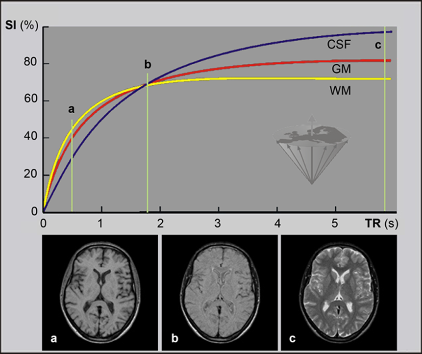
Figure 10-02:
Relative signal-intensity (SI) behavior of a partial saturation pulse sequence showing the dependence of SI of white matter (WM), gray matter (GM), and cerebrospinal fluid (CSF) at B₀ = 0.5 T.
If the repetition time chosen is long enough, signal intensities differ by the factor of proton density only (WM: 72%, GM: 82%, CSF: 100%). The images are of a healthy adult brain.
Simulation software: MR Image Expert®

Figure 10-02-Video:
In this animation we fly along the time line of the graph above and watch how the contrast changes.
Simulation software: MR Image Expert®
In general, bright regions on a PS image resemble object areas of short T1 and/or high proton density, while dark regions depict areas of long T1 and low proton density.
Hardly anybody uses the original PS sequences today because of their limited diagnostic value.
However, partial saturation becomes a gradient-echo sequence when a field gradient is added. Most sequences dubbed saturation recovery today are in reality gradient-echo sequences.
The principle elements of a spin-echo (SE) sequence are a 90° pulse followed by a 180° pulse after a time interval τ which builds up a spin echo after another time interval τ (2τ = TE, the echo time). The details were explained in Chapter 4.
Signal decay depends on the relaxation times and on ρ of the respective tissue. The curves reach zero signal intensity faster or slower, owing to the composition of the tissue (Figure 10-03).
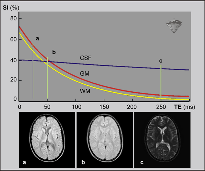
Figure 10-03:
Spin-echo sequence: decay curves of gray matter (GM), white matter (WM, and cerebrospinal fluid (CSF) at high field strength (B₀ = 1.5 T).
Relative signal intensity, SI, versus echo time, TE, at a given repetition time of TR = 2000 ms. The images are of a healthy adult brain.
Simulation software: MR Image Expert®

Figure 10-03-Video:
In this animation we fly along the time line of the graph above and watch how the contrast changes.
Simulation software: MR Image Expert®
When researchers in the early 1980s started applying the spin-echo (SE) sequence for medical imaging, they found better contrast but also more complicated contrast behavior. Some already known brain lesions were not seen because there was a lack of contrast. In particular, SE images with a TE shorter than 60 ms sometimes did not reveal multiple sclerosis plaques, astrocytomas, meningiomas, infarctions, or other lesions.
The reason for this behavior can be explained by the signal decay curves of spin-echo sequences. The signal intensity of different compounds decreases with longer TE. The most interesting features of these curves, however, are the points of intersection.
At these points, the respective brain tissues are isointense and there is no contrast between them: they are indistinguishable. Many pathologies possess signal intensities similar to normal brain tissue on images and therefore are invisible on images with short TE (T1 and intermediately weighted images).
The spin-echo signal contains information about proton density as well as spin-lattice and spin-spin relaxation. Signal intensity of a spin-echo sequence can be calculated by the following equation:
Again, SI stands for signal intensity, K represents the influence of flow, perfusion and diffusion, ρ is proton density, TR repetition time, TE echo time, and T1 and T2 are the relaxation times.
This equation reveals that T2-weighting of an SE image increases as the echo time advances. T1-weighting of the signal intensity depends on both TR and TE.
Figures 10-04a and 10-04b explain with two examples the interdependence of the echo time and the repetition time upon signal intensity and signal contrast.
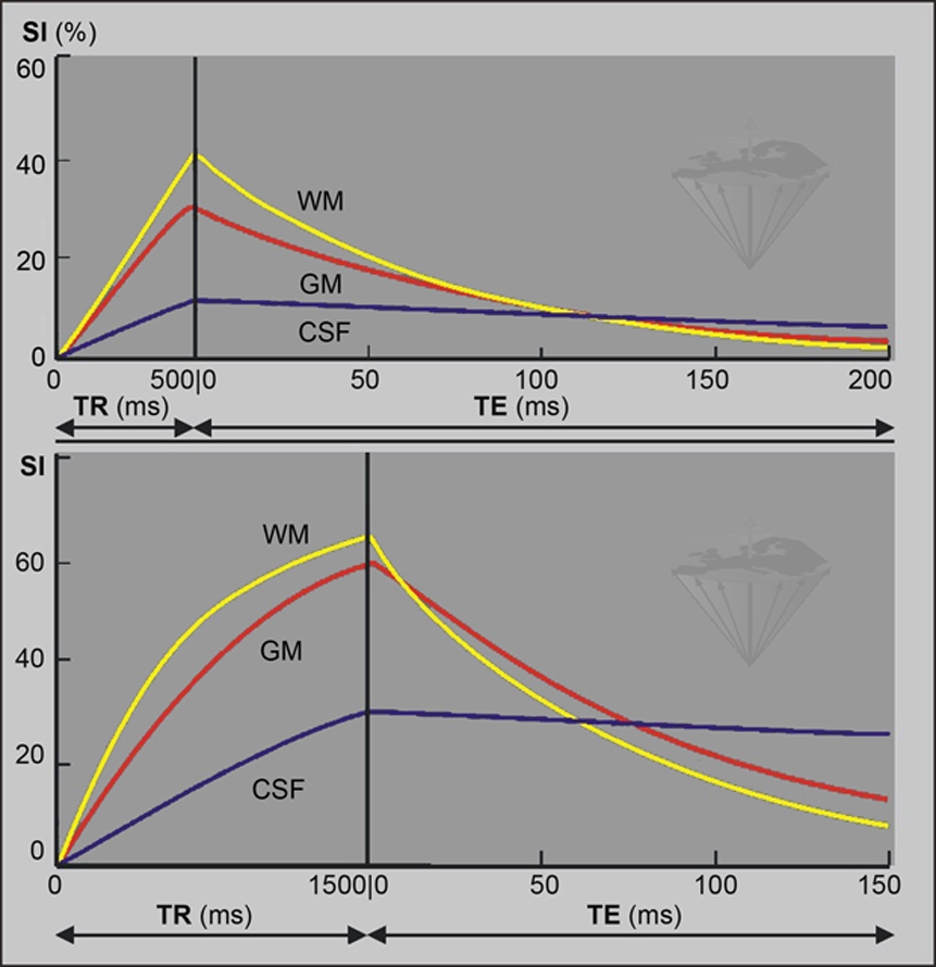
Figure 10-04a:
Top: Short repetition times (TR = 250 ms) emphasize T1-weighting.
Bottom: Long repetition times (TR = 1500 ms) emphasize T2-weighting. In brain imaging, the crossover points of no contrast move to shorter TE values when TR is increased.
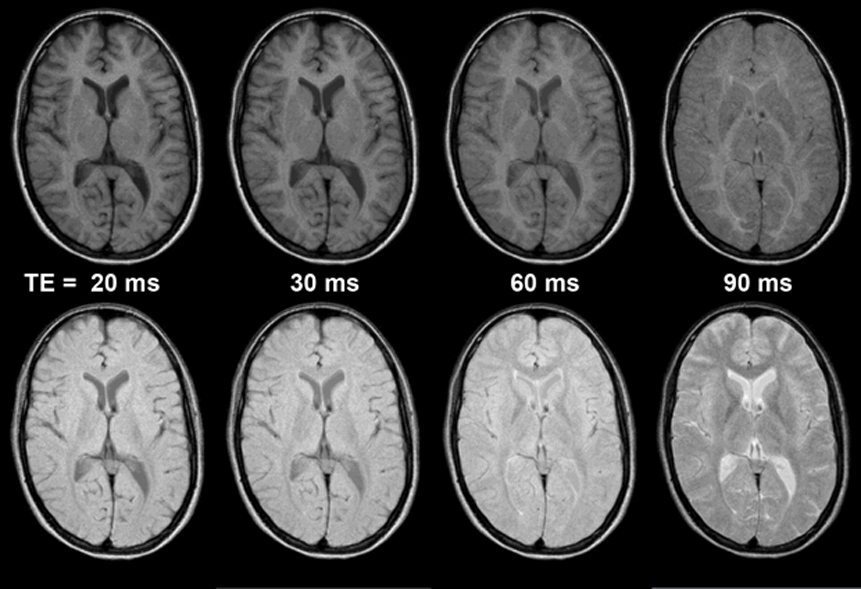
Figure 10-04b:
Spin-echo sequences: Echo times (TE) from left to right: TE = 20 ms, TE = 30 ms, TE = 60 ms, TE = 90 ms. B₀ = 1.5 T.
Top: Short repetition times (TR = 250 ms) emphasize T1-weighting.
Bottom: Long repetition times (TR = 1500 ms) emphasize T2-weighting. In brain imaging, the crossover points of no contrast move to shorter TE values when TR is increased.
Simulation software: MR Image Expert®
In a single echo SE sequence, T1-weighting usually is created by both short TR and short TE. In general, the early echoes (= short TE) of an SE sequence are ρ- and T1-weighted. The later echoes are increasingly intermediately and then T2-weighted.
When a short TR is chosen, the initial signal intensity will be low and SE images with short echo times will be heavily T1-weighted. With longer repetition times, signal intensities will be higher.
The relation of signal intensities to each other changes depending on TR, and thus contrast is also strongly influenced by TR.
Contrast might be predictable with normal anatomy; however, when searching for lesions, prediction may become impossible. Figure 10-05 gives an example of how a pathology can stay hidden or be highlighted.
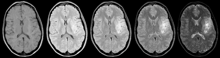
Figure 10-05:
The necessity of image acquisitions with different pulse sequence parameters: Brain, transverse view. SE sequence: TR = 1500 ms; TE from 15 ms to 225 ms. B₀ = 0.5 T.
On the more T2-weighted images, there is a clearly visible lesion: an old brain infarction. If you would just perform a T1-weighted study, only very suspicious radiologists will describe possible pathological changes: there is a slight mass effect.
Simulation software: MR Image Expert®

Figure 10-05-Video:
In this animation we fly along the time line given above and watch how the contrast changes.
Simulation software: MR Image Expert®
Sometimes the signal-decay curves of different tissues cross each other, leading to a complete extinction of contrast between them. The best contrast is seen when the relative ratio between them is highest. If the parameters (i.e., T1, T2, ρ, TR and TE) are known, the decay curves can be precalculated within a certain error range. However, if one does not know T1, T2 and ρ and uses the wrong pulse sequence parameters, one can overlook a lesion.
As we have seen in Chapter 4, one must clearly distinguish between T1- and T2-images ('pure T1- and T2-images') on the one hand, and T1-, T2- and intermediately (proton-density) weighted images on the other.
Whereas in the former images calculated relaxation times are depicted, the latter images show signal intensities with, e.g., in the case of a T1-weighted image, a high influence of T1, but at the same time also with T2 and proton-density contributions.
Table 10-02 gives an approximation to image weighting of SE sequences. Short TE and TR emphasize T1 influence, long echo and repetition times emphasize T2 influence. The combination of long repetition times and short echo times eliminate part of the T1 and T2 effects, thus emphasizing ρ.
Table 10-03 depicts the signal intensity behavior in 'weighted' spin-echo images. These image characteristics hold only for original SE sequences. They can be completely different in black box pulse sequences.
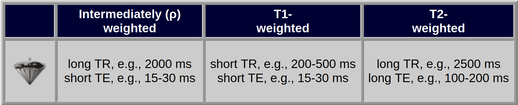
Table 10-02:
Spin-echo sequences: image weighting. Proton density (ρ-) images should preferably be called intermediately weighted images, because the highest signal intensity in these images might not present the highest water content.
TR and TE depend on field strength. At high fields, TR and TE for both T1- and T2- weighting are shorter than at medium or low fields.
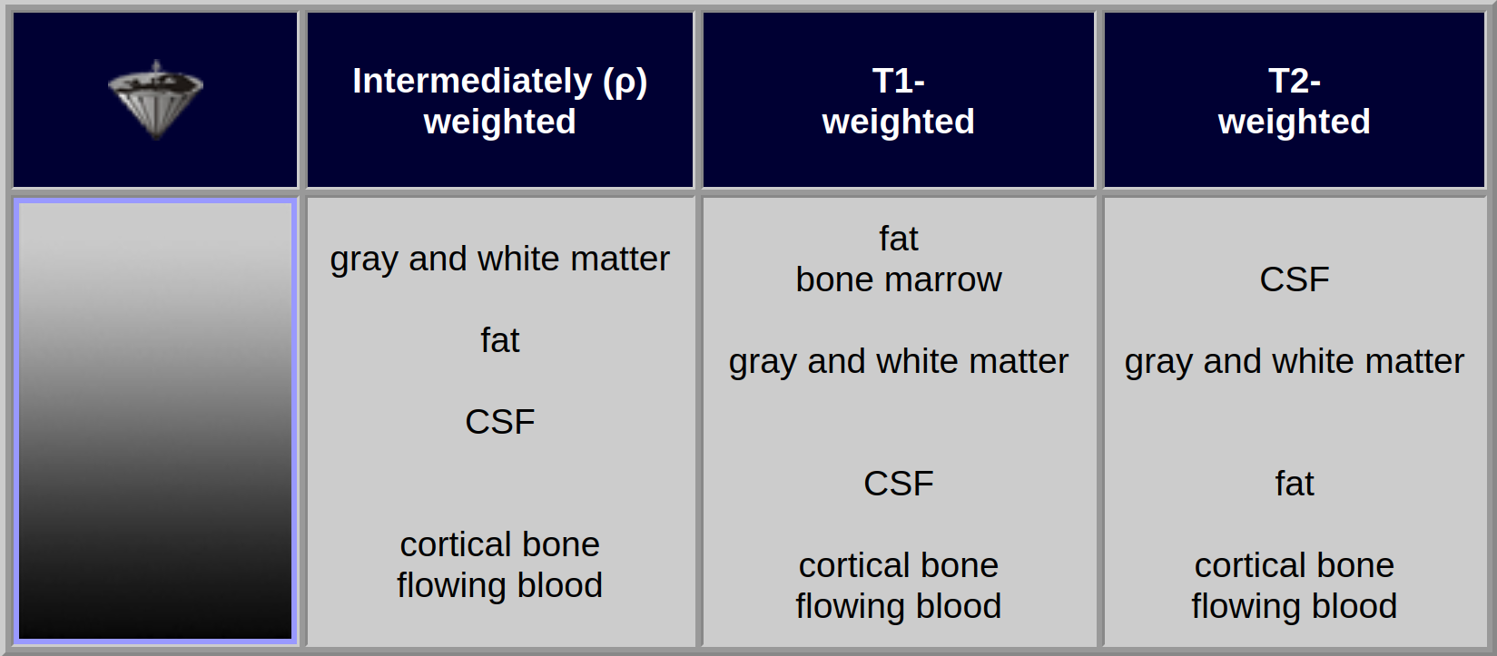
Table 10-03:
Spin-echo sequences: signal-intensity behavior of the brain in weighted images. Only weighted spin-echo images are used in routine clinical examinations. Within certain limits, their contrast behavior is reproducible, even with machines of different manufacturers. Today most machines use manufacturer-dependent ('black-box') pulse sequences.
Note that the respective signal intensities on weighted images vary according to the TE and TR chosen and with the strength of the magnetic field. The easiest way to distinguish T1- and T2-weighted images is by looking at water-like liquids: on T1-weighted images, they are dark; on T2-weighted images, they are bright.


|

|
|---|